
Overview
Nobody notices a 30% regression in a job whose runtime already swings ±20% between runs. The first slow run looks like noise. The fifth one looks like Tuesday. By the time someone files a ticket, the regression has been burning compute for weeks and the run that introduced it has aged out of everyone’s memory.
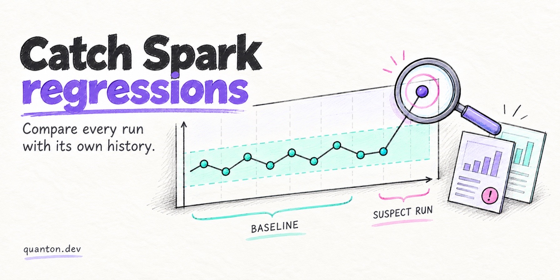
The only reliable defense is baselining: comparing every run against the job’s own history instead of against a human’s recollection of “how long it usually takes.” This post covers where regressions come from, how to compare runs with the Spark History Server, how to tell a real regression from normal variance with a P50/P95 baseline you can build in an afternoon — and how the Quanton agent turns any flagged run into a stage-level diagnosis.
Why did my Spark job get slower after an upgrade?
Because upgrades change plan choices, not just library code. The same SQL against the same data can compile to a different physical plan on a new Spark or Databricks Runtime version — and the plan is where the runtime lives.
The classic report reads like a StackOverflow post: “ETL job 3× slower after Databricks Runtime upgrade, no code changes.” No code changed. But underneath:
- AQE thresholds and defaults shift between versions. Adaptive Query Execution decides at runtime whether to coalesce partitions, convert joins, or split skewed partitions — and the thresholds driving those decisions (
spark.sql.adaptive.autoBroadcastJoinThreshold, advisory partition sizes) have changed defaults across Spark 3.x releases. - Join strategies flip. A join that used to broadcast falls back to sort-merge because a size estimate crossed a threshold, or the reverse — a forced broadcast now OOMs the driver. Either direction can dominate a job’s runtime; the SHJ vs SMJ deep dive covers why the gap is so large.
- Optimizer rules change stage shapes. New rewrite rules move filters, collapse or introduce exchanges, and change how many shuffle boundaries the job crosses.
And it isn’t only upgrades. Data growth pushes size estimates past optimizer thresholds. Input layout drift — small files accumulating, clustering decaying — inflates scan stages. Cluster changes (instance types, autoscaling policy) alter the hardware assumptions the old runtime was tuned for.
How to confirm a plan regression: diff the physical plans of a known-good run and a slow run. If the plans differ — a join node changed type, an exchange appeared, a scan lost its pushed filters — you’ve found the mechanism, and you can pin it to the version or config change between those two runs. The History Server keeps the SQL plan for every completed run, so the evidence is already there; fetching the two plans is your legwork. The plan forensics isn’t: on Quanton, the AI agent has the current run’s SQL plan in context — ask it why the join stopped broadcasting, or paste the old plan into chat, and it names the flip and its likely trigger.
How do I compare two Spark job runs?
The manual way: open both runs in the Spark History Server, side by side in two tabs, and diff them stage by stage — duration, task count, shuffle read/write bytes, spill, input size. Then open the SQL tab in both and compare the physical plans by eye.
It works. It’s also tedious and error-prone in exactly the ways that matter:
| Manual SHS diff | Why it fails in practice |
|---|---|
| Stage IDs don’t line up across runs | AQE re-plans at runtime, so “stage 14” in run A isn’t stage 14 in run B |
| Two tabs, dozens of stages | You’ll compare the three stages you suspect and miss the one that regressed |
| No history, only pairs | Comparing against one prior run can’t tell you whether either run was normal |
| Plans are trees rendered as text | A flipped join three levels deep is easy to scroll past |
Two upgrades make it tractable. First, script the cross-run half — the part no tool does for you. The SHS REST API (/api/v1/applications, plus per-application stage endpoints) exposes every run’s duration and stage metrics as JSON; a short script that appends each run’s numbers to a table gives you cohorts instead of pairs, and comparisons against the job’s history instead of one arbitrary previous run.
Second, hand the suspect run to the Quanton agent for the per-run half. This isn’t a special feature — it’s the model reasoning over the same tool data you’d read by hand: with the run’s stages, tasks, SQL plans, and executor logs in context, it attributes the compute to stages (“the join in stage 23 consumed the extra executor-seconds, not the scan”), separates skew from stragglers from GC by the task-duration and shuffle-read distributions, and explains the plan. The stage-by-stage archaeology that eats the afternoon is exactly the part it’s good at.
Is this run normal, or a regression?
A run is a regression signal when it falls outside its cohort’s P95; inside the P50/P95 envelope, it’s noise. That’s the entire test, and it’s why baselining beats thresholds: “alert if runtime > 60 min” is wrong for a job whose healthy range is 20–70 minutes, and silent for a job that drifted from 10 to 55.
Envelope thinking gives you three distinct verdicts instead of one alarm:
| Signal | Looks like | Actually is |
|---|---|---|
| One run beyond P95, next runs back at P50 | ”The job broke” | One-off spike — spot reclaim, contention, a bad node. Investigate only if it repeats |
| Runtime jumps and stays at a new level after a specific date | ”It’s been slow lately” | Step-change regression — upgrade, config change, or plan flip on that date. Diff plans across the boundary |
| P50 itself creeps up over weeks, envelope intact | ”Feels slower than last quarter” | Slow drift — data growth, skew shifting, file layout decaying. Fix the data, not the code |
| Run lands below P50 after a change | Easy to ignore | Improvement — worth confirming and locking in, so the baseline tightens |
This is the part to automate yourself, and it’s smaller than it sounds: a scheduled script that pulls each completed run’s duration from the SHS REST API, computes P50/P95 per job, and flags runs beyond the envelope — plus median drift over a trailing window — is an afternoon of work. The payoff is the table above running continuously: slow drift surfaces even though no single run ever looked alarming.
Why is my Spark job runtime inconsistent?
Because the job’s environment isn’t constant, even when the code is. The usual sources of run-to-run variance:
- Input volume. Daily partitions aren’t the same size; Monday’s data isn’t Friday’s. Runtime tracking input size is variance, not regression.
- Skew moves with the data. A hot key that’s 2% of rows one day and 9% the next changes which task is the straggler — see the data skew deep dive for why one partition can dominate a stage.
- Spot interruptions and executor churn. Losing executors mid-stage means retried tasks and recomputed shuffle data — the same job does more total work some runs than others.
- Cluster contention. On shared clusters, your stage waits on someone else’s I/O or scheduler queue.
- Dynamic allocation ramp-up. A job that starts at 2 executors and scales to 50 spends its first minutes under-provisioned; how fast it ramps varies with cluster headroom.
Baselining is what separates this variance (scatter around a stable median) from drift (the median itself moving). You can’t do that from memory, and you can’t do it from the last run alone — you need the distribution. That’s exactly what the P50/P95 cohort gives you, and it’s also why “is this run expensive?” is a history question: the same attribution that explains a regression feeds the waste analysis in finding wasted Spark and Databricks compute.
The workflow: baseline every run
End to end, with the boundary drawn honestly — the history-keeping is a script you own; the run forensics is where the agent earns its keep:
- Export run history from the Spark History Server. The REST API (
/api/v1/applications) returns every completed run’s duration; per-application endpoints add stage-level durations, shuffle bytes, and spill. No job code changes — the data is already being written. - Compute the envelope. A scheduled script (or notebook, or dashboard query) computes P50/P95 runtime per job and flags any run beyond P95 — plus median drift over a trailing window for the slow-creep case.
- Triage a flagged run against the table above. One-off spike, step change, or drift? For a step change, pull the physical plans of the last good run and the flagged run and diff them.
- Hand the flagged run to the Quanton agent (if the job runs on Quanton). With the run’s stages, tasks, SQL plans, and executor logs in its context, ask the question you’d ask a teammate: “which stage consumed the extra compute?”, “is the straggler in stage 23 skew or a slow node?” — the answer names the stage and the mechanism, not a vibe.
- Confirm the mechanism, then fix. Plan flip → pin it to the version or config change between those runs; skew or layout decay → it’s a data-side fix; the Spark performance tuning guide covers what to tune once you know which stage to aim at.
How do I snapshot a run before and after a change?
For a quick, shareable artifact — say, proving a fix landed — run Spark Analyzer (Onehouse’s free CLI) against your Spark History Server before and after. Each run gets a report with wall-clock, compute used vs. wasted, and a stage-level breakdown; two reports side by side make a regression (or an improvement) concrete enough for a PR description.
pip install spark-analyzer
spark-analyzer configure          # point it at your Spark History Server
spark-analyzer analyze --save-local
It runs locally (--save-local keeps data in your environment). Example reports are in the Spark Analyzer walkthrough.
Takeaway
Regressions don’t announce themselves; they hide inside variance. A fixed runtime threshold can’t see them, and a human watching a dashboard can’t hold fifty runs of history in their head. Baseline every run against its own P50/P95 cohort, diff plans across any step change, and attribute slow runs to stages — the History Server already has all the data, and the baseline script is an afternoon of work that pays out every week after. On Quanton, the agent then turns any flagged run into a stage-level diagnosis in minutes instead of an afternoon.
