Agentic AI

Quanton embeds an AI agent directly into the Apache Spark Web UI. While your job is running, it analyses stages, tasks, executor metrics, SQL plans, and — when you connect a Spark History Server — your prior runs of the same job. Then it surfaces answers, alerts, and cost findings in plain English.

No changes to your job code. No external tooling. Just open the Spark UI.

Enable the agent

Starting with Quanton Operator 2.0, the agent ships with the operator. Two ways to turn it on.

Option 1: Operator-wide (recommended)

When installing the operator, set onehouseConfig.enableAIAgent=true. Every QuantonSparkApplication submitted afterwards picks up the agent automatically — no per-job config.

helm upgrade --install quanton-operator oci://registry-1.docker.io/onehouseai/quanton-operator \
    --namespace quanton-operator \
    --create-namespace \
    --set "quantonOperator.jobNamespaces={default}" \
    --set onehouseConfig.enableAIAgent=true \
    -f onehouse-values.yaml

Option 2: Per-job

If you want the agent on for some jobs but not others, leave the operator default off and add one Spark config to your QuantonSparkApplication:

spec:
  sparkApplicationSpec:
    sparkConf:
      spark.quanton.agent.enabled: "true"

Open the agent UI

Once the driver pod is Running, port-forward to it:

kubectl port-forward <driver-pod-name> 4040:4040 -n <namespace>

Open http://localhost:4040. The AI Agent button appears in the bottom-right corner of every Spark UI page.

Settings — connect a provider and (optionally) a Spark History Server

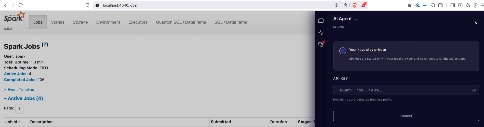
Click the AI Agent button, then Settings. There are two things to configure.

LLM provider + API key

Paste your key. The provider (Anthropic, OpenAI, or Google Gemini) is auto-detected from the key prefix. The model picker then populates with the models your key can access.

Provider	Models we've validated
Anthropic	claude-opus-4-7, claude-sonnet-4-6
Google Gemini	gemini-2.5-pro, gemini-2.5-flash
OpenAI	gpt-4o, gpt-4.1

Any other model your provider exposes will also appear — the list is fetched live from the provider.

Your API key is stored in your browser's localStorage. It never reaches Onehouse servers. The agent makes its LLM calls directly from the driver pod to your provider over HTTPS using the key you pasted.

Spark History Server (optional, but recommended)

Pasting a Spark History Server URL unlocks the agent's most useful capability: comparing the running job to its own past runs.

http://spark-history.<namespace>.svc.cluster.local:18080

The Settings page validates the URL by probing it from the driver pod (not your browser), so a kubectl port-forward localhost URL reachable from your laptop won't work — use a cluster-internal URL.

With SHS connected, the agent automatically:

• Identifies prior runs of the same logical job (across renames, restarts, and orchestration churn).
• Computes a baseline envelope (P50 / P95) for runtime, shuffle, spill, GC, executor count.
• Flags whether this run is normal, a regression, or an improvement — and against which past run.
• Powers the Cost tab's history-anchored findings (see below).

Without SHS the agent still works, but every finding is grounded in just the current run.

What it does

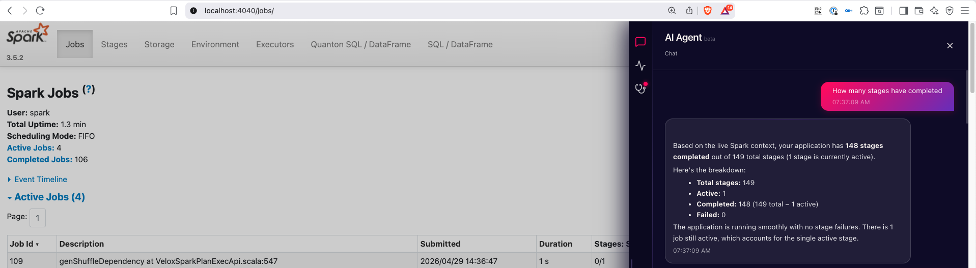
Chat

Ask questions in natural language. The agent has full context — stages, tasks, SQL plans, executor logs, alerts — and answers about your job, with deep links back into the Spark UI.

"Why is stage 4 taking so long?" "Which executor is causing the skew?" "Is this run slower than usual?" (needs SHS) "What changed between this run and yesterday's?" (needs SHS)

A few chat conveniences:

• @ mentions. Typing @ opens a typeahead for jobs, stages, executors, SQL queries, and failed tasks. Mentioning an entity narrows the agent's context to that thing.
• Slash commands. Type / to pick a skill — /spark-debugger for failure-focused triage, /performance-tuner for slowdown analysis.
• Per-app history. Chat persists per application across Spark UI navigation. Closing a tab and coming back keeps your conversation.

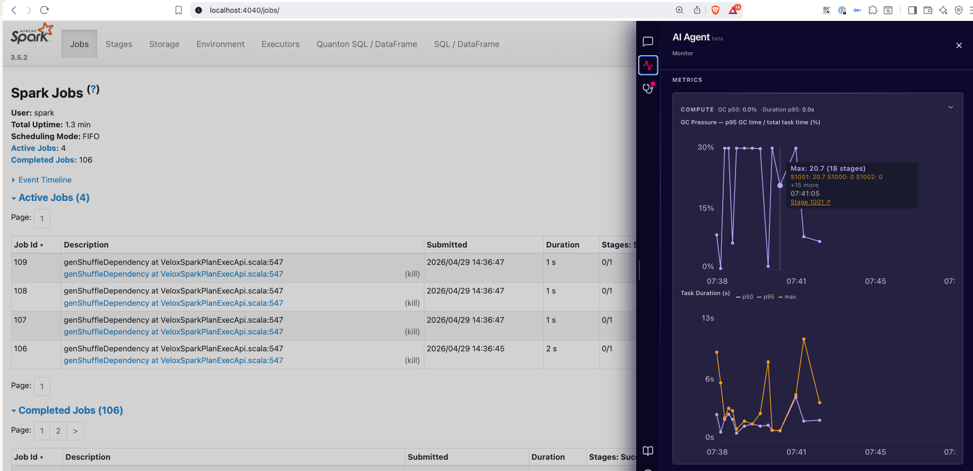
Monitor

Live executor and SQL metrics on a 2-second refresh while the tab is visible:

• GC pressure — fraction of executor time spent in garbage collection.
• Skew ratio — how unbalanced task durations are within a stage.
• Spill — total memory + disk spill across active stages.
• Task duration — per-task runtime distribution, with stragglers highlighted.
• Shuffle — bytes read/written, partitions, fetch wait time.
• Executor info — CPU, heap, active/failed task counts per executor.

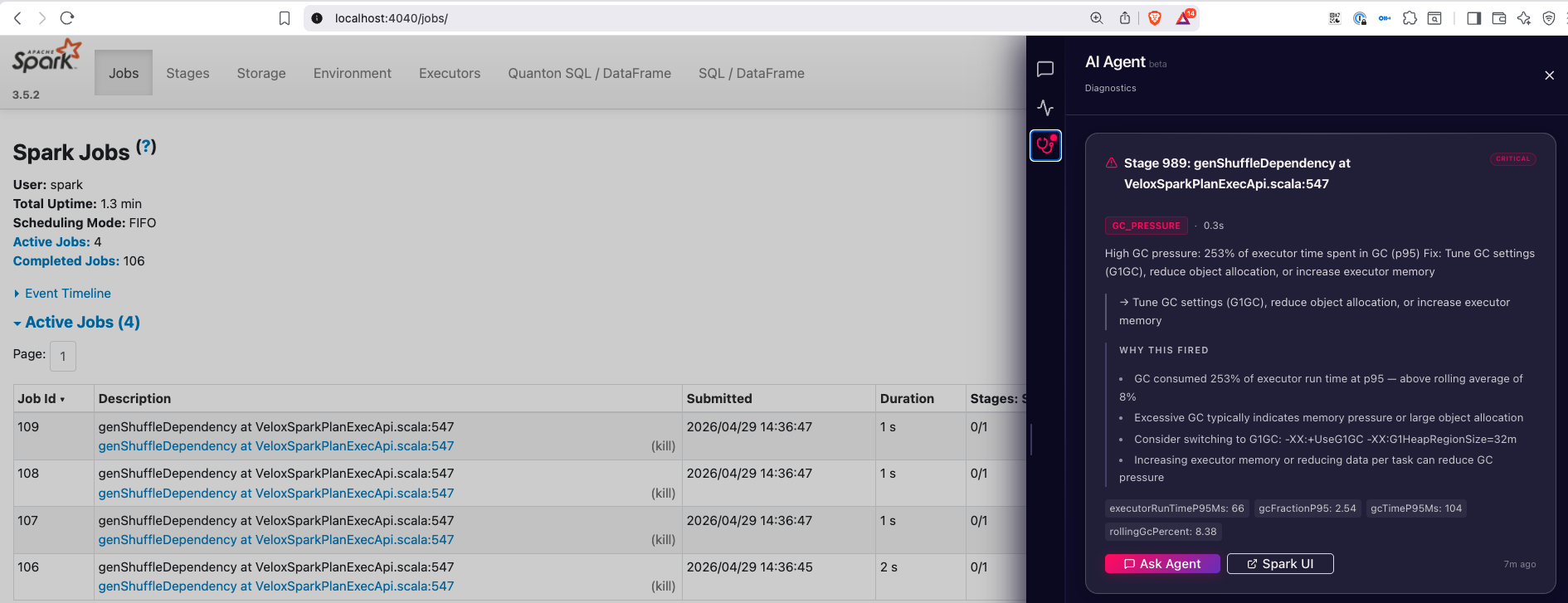
Diagnostics

Real-time health alerts for the conditions that slow Spark jobs down most. Each alert shows the underlying numbers, the affected stage, and an Ask Agent button that opens Chat pre-loaded with the alert context.

Detects:

• Data skew (task duration, shuffle read, record count)
• Memory and disk spill
• GC pressure
• Out-of-memory failures
• Straggler tasks
• High shuffle fetch-wait
• Shuffle-write explosion (shuffle ≫ input)
• Partition sizing (too many small / too few large)
• Failed task clusters
• Executor churn

Savings

The Savings tab ($ icon in the sidebar) is separate from Diagnostics, and the two answer different questions:

• Diagnostics tells you what's wrong with a specific stage right now — a per-stage, per-event alert stream.
• Savings tells you what fraction of the whole run's compute was wasted, and on what — a job-wide accounting with a "where can I cut?" framing.

They share underlying signals (a skew alert in Diagnostics often shows up as skew_cost in Savings), but Diagnostics surfaces the symptom as it happens while Savings rolls everything up against an executor-seconds denominator.

Everything in the Savings tab is expressed in executor-seconds and percentages — never a dollar amount, because dollars depend on instance type, region, and commitments the agent can't see. Multiply executor-seconds by your own hourly rate if you want a USD estimate.

Headline

The top tile leads with the absolute number of executor-seconds recoverable on this run, with the percentage of total allocated compute as a secondary stat. A horizontal bar shows the split between useful and wasted executor-seconds.

A confidence pill on the right tells you what the headline is grounded in:

• Cohort-grounded — Spark History Server is connected and the agent found comparable prior runs to baseline against.
• Live data only — no SHS, no comparable history, or SHS unreachable. Findings still surface, but without "vs baseline" framing.

Findings

Below the headline, each contributing category renders as a collapsible row: severity dot, name, a "save up to N exec-sec" pill, and the impact %. Click a row to expand and see the evidence, a copy-ready fix snippet, and the underlying sources. Categories include:

• Over-provisioning — executors held but not running tasks.
• Idle executors — provisioned but never assigned work.
• Dynamic-allocation churn — executors decommissioned within seconds of being spawned.
• Straggler tax — stage held open by one slow task.
• Skew cost — uneven partitioning forcing serial work.
• Retry overhead — task retries from transient failures.
• Spill cost — executor-seconds spent spilling to disk.
• GC overhead — executor-seconds spent in garbage collection.
• Speculative waste — duplicate speculative executions that lost the race.
• Plan regression — slowdown attributable to a query-plan change.
• Failed-task overhead — work redone after task failures.

Findings below 3% impact collapse into a "small findings" expandable row, so the headline view stays uncluttered.

Severity tiers (in headline + finding rows):

Tier	Threshold
Critical	≥ 15%
High	5 – 15%
Medium	3 – 5%
Minor	< 3%

When SHS is connected, findings include a [history: …] citation showing how this run compares to your past runs of the same job.

Run Comparison

When SHS is connected, a Run Comparison tile sits below the headline with two views you can toggle between:

• Rank — bar chart of cohort runs sorted costliest → cheapest by executor-seconds, with this run highlighted in pink. The big number tells you ±% vs the cohort median and where you rank (e.g. "+22% · ranked 4 of 12"). Hover any bar to see its app id and delta vs the current run; click to copy the app id.
• Timeline — chronological sparkline across the cohort. If the linear fit is strong enough (R² ≥ 0.30 with 8+ runs), a headline calls the direction (e.g. "↑ 6%/week"). Otherwise it explicitly says "No reliable trend" rather than fit a line to noise.

Each view has an Ask Agent button that opens Chat with a contextual question already typed — comparing this run to the cheapest cohort run, or identifying when a trend started.

Compute Attribution by Stage

Below Run Comparison, the Compute Attribution by Stage tile shows the top stages by executor-seconds, each annotated with a dominant-factor label (e.g. SKEW, SPILL, GC_PRESSURE) when a Diagnostics rule fired on that stage. This is unconditional compute attribution — a stage shows here based on share of executor-seconds, whether or not it tripped a rule. The Ask Agent button on this tile opens Chat with a question that drills into the hottest stages.

Loading behavior

The headline + findings render in under a second from live data. If SHS is configured, the Run Comparison tile loads in the background (typically 10–25s) and the confidence pill upgrades from "Live data only" to "Cohort-grounded" as cohort data lands.

Cost questions in Chat

The agent can also answer cost-shaped questions directly in the Chat tab. A few examples:

"Summarise this run's cost." — Returns the top contributors, total waste, and a one-line headline. "What would I save if I dropped to 8 executors?" — Projects waste reduction from a hypothetical cluster shape, using the cohort to bound the estimate. When the projection model doesn't fit your dominant waste shape (e.g. you're spill-bound, not over-provisioned), the agent says so rather than make up a number. "Is my GC time trending up?" — Flags persistent upward slope in gc_time_ms or shuffle_read_bytes across the cohort, only when the slope is statistically significant.

Keep the driver alive after the job ends

By default the Spark UI (and the agent) disappear when SparkContext stops. For post-mortem inspection, enable await-termination:

spec:
  sparkApplicationSpec:
    sparkConf:
      spark.quanton.agent.enabled: "true"
      spark.quanton.agent.await.termination: "true"

When the job ends, a banner appears in the sidebar with two buttons:

• Allow termination — releases the driver, JVM exits, pod terminates.
• Extend — resets the countdown.

The driver auto-terminates 30 minutes after job-end by default — enough time to investigate, short enough that forgotten sessions don't pile up pods. Override with:

spark.quanton.agent.await.termination.timeout: "1h"   # any Spark duration string
spark.quanton.agent.await.termination.timeout: "0"    # disable auto-termination (manual dismiss only)

Try it on a real workload

The operator repo ships a self-contained TPC-DS example with the agent enabled. 1000+ stages, 99 SQL queries, real shuffle and join activity — a meaningful workload for the agent to reason about.

git clone https://github.com/onehouseinc/quanton-operator
cd quanton-operator/examples/tpcds-agent
./run.sh                        # default — SF=10 (~10–15 min datagen, ~8–30 min queries)
# or smaller for a quick demo:
SCALE_FACTOR=1 ./run.sh         # ~3–5 min datagen, ~2–3 min queries

See examples/tpcds-agent/README.md for prerequisites and details.

Notes

• The agent UI is reachable only while the driver pod is running. When SparkContext shuts down at job end, the Spark UI (and the agent) go with it — unless you've enabled await-termination above.
• For short jobs, the UI may disappear before you can interact with it. Run a bigger workload (SCALE_FACTOR=10 or higher in the example), or enable await-termination.
• The agent never sends your code, data, or query results to Onehouse. It runs entirely in the driver pod and talks only to the LLM endpoint you configured.